Approximate Bayesian Computation (ABC)
Mathematical Visualizations
Introduction
This project aims to create an “explorable explanation” for the Approximate Bayesian Computation (ABC) algorithm.
1. Approximate Bayesian Computation (ABC)
This is an algorithm created to estimate the posterior probability density. Originally, it was proposed as a way of explaining how posterior probabilities could be understood in the context of frequency sampling. The idea originated from a paper of Donald Rubin in the 1980′s, which stated that a posterior can be obtained by choosing parameters from a prior, simulating the sampling process of the real observations and accepting the parameters only when the simulated sample matched the real one. This method is also called likelihood-free, since it allows one to obtain a posterior probability without the use of the likelihood function. Such feature is very important in problems where the likelihood function has an unknown closed form or is very expensive to calculate.
1.1 ABC Original Algorithm
The idea of the ABC sampler is that we can get the posterior probability density function by samping from the prior distribution and then simulating the statistical experimenting, accepting the sampled parameter when the simulation result matches with the observed real world experiment.
Perhaps a better way to understand the method is with an example. Assume that we threw a coin 8 times and observed 6 heads. Supposing that the bias of our coins (θ) come from a uniform prior distribution, we want to get the posterior distribution.
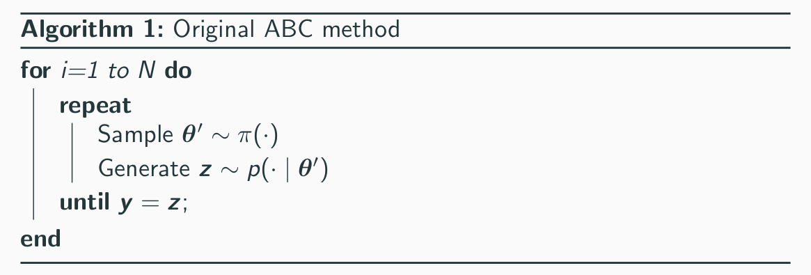
This posterior distribution can be obtained in the following way. First, we sample a coin with bias θ from the prior distribution π(θ). We then throw the coin 8 times and check how many heads (sucesses) we got. If the number of heads is equal to 6 (the observed value), then we accept the θ. After doing this several times, the distribution of the θ’s accepted is equal to our posterior distribution. The algorithm for the method is shown below.
Let’s run a simulation!
We start with the sample 1. Running the simulation:
- Coin has a θ = 0.891894;
- Simulated number of heads = 7 ;
- Coin Rejected
To simulate more samples at once, use the handle above.
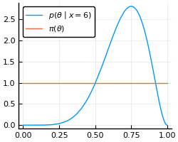
In the case above we obtain the posterior distribution only for the case when K=6. This is extended in the graph below. In the left we plot all the coins sampled with the respective number of heads obtained when the throws are simulated. At the right we plot the histogram of the bias (θ) of this coins by filtering by the number of heads obtained.
This graph is interactive, hence, you can alter the gray region which filters the coin by number of successes. Changing the position of the filter, one can observe the different posterior distribution estimates given by the ABC sampler for different observed number of heads.
1.2 ABC for Continuos Variables
Pritchard et al. (1999) extended the original algorithm to the case of
continuos sample. The problem with continuos variables is that
a precise match between the simulated and the observed value becomes impossible.
The intuitive extension of the model is use a precision distance (ϵ), so
we accept θ when the simulated and the observed value are closer than a value
ϵ. Another extension is to use a sufficient static instead of each individual
observed value.
The algorithm for ABC dealing with continuos variables
is given below.
 Again, let’s do an example to make the method clearer.
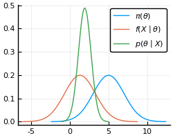
Consider a model where and , with
known. Therefore, our posterior distribution is also gaussian.
Again, let’s do an example to make the method clearer.
Consider a model where and , with
known. Therefore, our posterior distribution is also gaussian.
In our toy model, we observed 5 values with the mean equal to 1.3. The mean is a sufficient static for this model, hence, our algorithm works by sampling a θ from the prior, then we use this θ to sample 5 values from and take their average. If the distance between the synthetic average and the observed average is less or equal than ϵ, we accept the θ.
In the graph below we plot the synthetic average for each simulation. The gray area represents the acceptance region and the green line is the observed average. You can vary ϵ and see how decreasing it leads to a better approximation of the posterior. You can move the range slider to change the starting value of the threshold 3.00.
ϵ : 0.1 10
1.3 ABC Post-Processing
As models grow in complexity, the threshold (ϵ) starts to become a problem, since we need lower and lower values to get a better approximation, this increases the number of simulations that we need to performed. A solution to this problem using linear regression was proposed by Beaumont et al. (2002). The method is a way to improve the results of the simulations without the need to use restrictively low threshold values.
The idea is to “estimate” the value of θ by projecting the sampled values in the axis where the error (observed vs. simulated) is equal to zero. Thus, allowing us to use sampled value of θ even when the error is quite significant. The original model by Beaumont et al. (2002) uses a weighted regression and considers only the values up to an error where a linear regression seems appropriate. In our toy model, we actually use a non-weighted regression and all the simulated samples (which is ok since we are in a fairly simple model).
In the graph below, the pink line is the linear regression and the green points are the projection of each blue point in the y-axis. The histogram in the right uses these projected points to construct the approximation of the posterior. You can pass your mouse over the scatter plot to see the corresponding projection of each point, and double click to deselect all points.
Conclusion
The ABC algorithm is not only an insightful way of understanding how to generate posterior distributions, it is also a useful method when one does not want to compute the likelihood to obtain the posterior distribution. The algorithm worked very well for both of our examples, but as models get complex, obtaining good approximations starts to become a challange, specially due to the lack of low-dimensional sufficient statistics and the need to use decreasingly low thresholds. We presented one of the methods used to improve the results of the ABC algorithm, the local linear regression method. This method worked quite well to avoid the need of using a very low threshold to get a good approximation for the posterior.
ABC methods are still in active research. Here can be found a presentation containing a more thorough review of the topic.
This article was created using Idyll, with visualizations powered by Vega-Lite. The source code is available on GitHub.
References
Beaumont, M., Zhang, W., and Balding, D. (2002). Approximate bayesian computation in population genetics. Genetics,162(4):2025–2035. ID number: ISI:000180502300043.
Pritchard, J. K., Seielstad, M. T., Perez-Lezaun, A., and Feldman, M. W. (1999). Population growth of human Y chromosomes: a study of Y chromosome microsatellites. Molecular Biology and Evolution,16(12):1791–1798.
Rubin, D. B. (1984). Bayesianly justifiable and relevant frequency calculations for the applied statistician. Ann. Statist.,12(4):1151–1172.